
Browse All Articles > A matter of highlighting in Excel
I have seen some great articles online relating to how can we highlight a cell or range of cells based on certain criteria, whether it's using simple conditional formatting or with the help of macro scripts. In this article, I discuss some of these implementations.
Highlighting in Excel is important, and in fact, we may need to use this technique to make our task easier in our daily operations at work.
Here are a few use cases.
1. Highlight in basic ways
2. Highlight an active row and column
3. Highlight duplicate values in the same column(s) based on the active cell
1. Highlight in basic ways
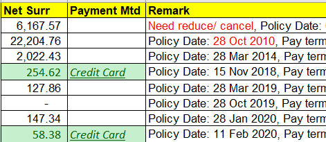
a) Very basic highlighting
From the Home tab, we can use the Font, Alignment, Number, and Styles functions to format a range of cells we have selected.
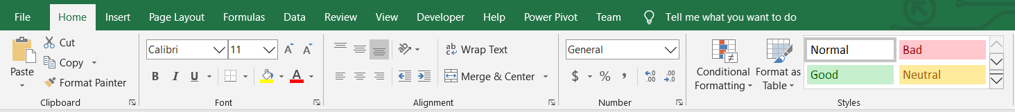
That's where we can create basic formatting in Excel.
For example:
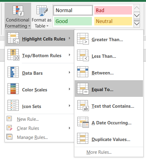
b) Conditional Formatting
Conditional Formatting is one of the features available in the Styles function.
There are some predefined rules, such as Equal To, Greater Than, Less Than, etc. available, that we can simply select to apply a format accordingly.
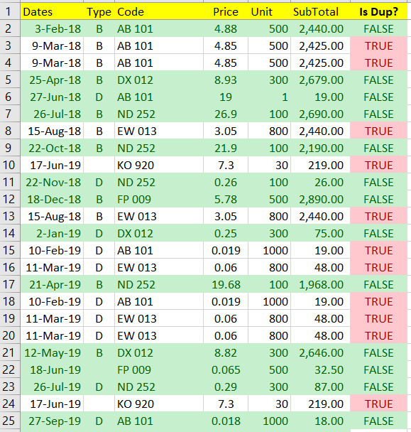
In my previous article: Handling Duplicate Rows In Excel, I mentioned how we could easily apply Conditional Formatting to highlight duplicate values.
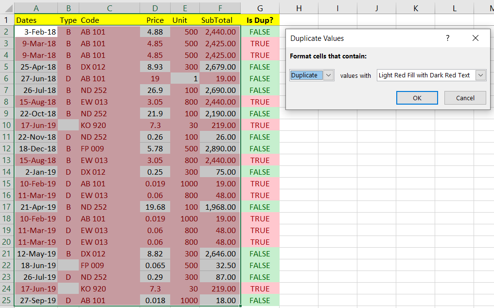
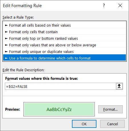
We can also use the Formula Formatting Rule to highlight duplicate rows.
2. Highlight an active row and column
a) Conditional Formatting
By applying the solution of this EE question: Is there a way to change the accentuation of the row and column highlights in Excel 2016?
We can create a Conditional Formatting rule with a formula to highlight the row and column active cells.
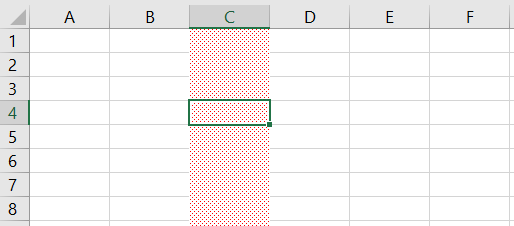
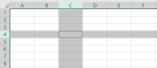
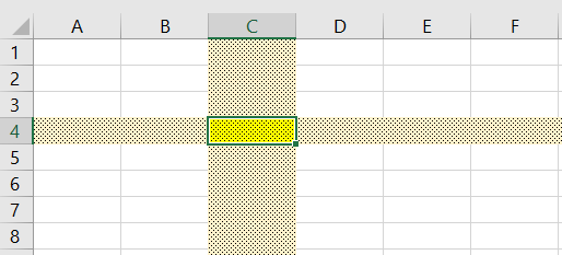
For example, if Cell C4 is selected, row 4 and column C should be selected.
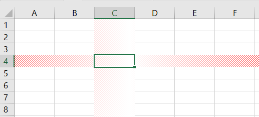
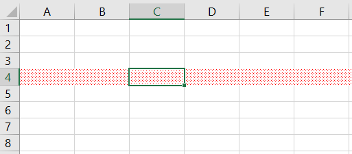
In order to highlight the row only for a similar effect, we can apply the following Formula:
The result will be like this:
In order to highlight the column only for a similar effect, we can apply the following Formula:
The result will be like this:
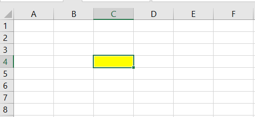
To change the active cell formatting alone, we can apply the following Formula:
The result will be like this:
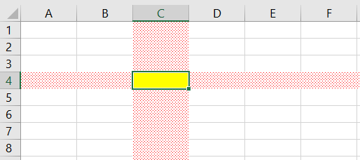
By combined these rules together, you could create something like below:
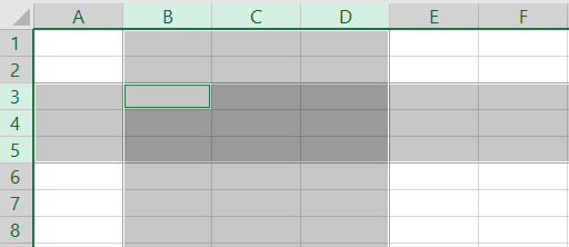
So far it looks pretty good for what we have done, but I have also spotted one issue if the selected cell is more than a single cell.
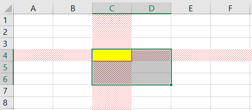
Can we prevent highlighting if multiple cells are selected? Or can we highlight multiple rows and columns for active cells?
This issue may not be able to be resolved by a formula, so we can use a Macro to resolve it.
b) Use a Macro
I'm referring to another EE question:
One of the comments that I found pretty useful was: Need Help with Excel (Row Highlighting)
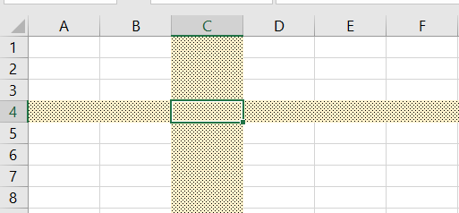
By applying the macro codes above, it creates the effect below:
By using the same codes, we can have rows and columns for selected cells to be highlighted as well.
This looks pretty good, but what if we want to customize the highlighting effect?
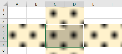
We can actually do that by customizing the macro codes like below:
By applying the above codes, we have created something like below:
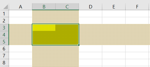
Selecting multiple cells are also supported with the same codes above.
In case we want to have different formatting for the selected cells, we can apply the following codes:
By applying the above codes, we are creating something like below:
Selecting multiple cells is also supported with the above same codes.
NOTE: However, as you may have found, the copy and paste function will no longer work after you apply the codes into your worksheet.
This happens because we are calling the ClearFormats method which also causes the copy and paste function to fail. To resolve this issue, we would need to replace that command with codes to update the interior properties.
The updated code should look like this:
This will generate the result similar to the previous example, but now we are able to do the copy and paste within the same worksheet.
3. Highlight duplicate values in the same column based on an active cell
Trying to highlight, we got this possibility which is based on a real scenario.
A use case that involves sending emails to a 3rd party person. I can determine how many emails I have sent out to a particular person by using the COUNTIF (or COUNTIFS) function in Excel.
But at the same time, I would like to know if it's possible to simply highlight the cells that have the same values as the current active cell.
Given an example below:
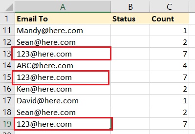
If I have the active cell at A19, can the cell A13, A15 and A19, and the rest of them with the same value be highlighted with a different color format?
I'm not too sure if there's a better way, but at this juncture, I came to a solution by using the Macro codes below:
This approach seems to be working well and created the effect I wanted.
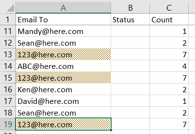
Selecting multiple cells is also supported with the same codes above.
NOTE:
i) I have built the logic so that empty cells will not be selected.
ii) I have set a Constant MAX_CELL_SELECT_CNT in the codes to set a threshold so that we can control the number of values to be looked up and prevent a heavy load such as in a scenario when one whole or multiple columns were being selected.
iii) DoEvents function was being added in the code so that we have a chance to pause the long process, just in case we did not handle it properly.
Hopefully, this article is useful to you.
You are encouraged and welcome to give me feedback for any possible improvements.
Here are a few use cases.
1. Highlight in basic ways
2. Highlight an active row and column
3. Highlight duplicate values in the same column(s) based on the active cell
1. Highlight in basic ways
a) Very basic highlighting
From the Home tab, we can use the Font, Alignment, Number, and Styles functions to format a range of cells we have selected.
That's where we can create basic formatting in Excel.
For example:
b) Conditional Formatting
Conditional Formatting is one of the features available in the Styles function.
There are some predefined rules, such as Equal To, Greater Than, Less Than, etc. available, that we can simply select to apply a format accordingly.
In my previous article: Handling Duplicate Rows In Excel, I mentioned how we could easily apply Conditional Formatting to highlight duplicate values.
We can also use the Formula Formatting Rule to highlight duplicate rows.
2. Highlight an active row and column
a) Conditional Formatting
By applying the solution of this EE question: Is there a way to change the accentuation of the row and column highlights in Excel 2016?
We can create a Conditional Formatting rule with a formula to highlight the row and column active cells.
For example, if Cell C4 is selected, row 4 and column C should be selected.
=OR(ROW(A1)=CELL("row"),COLUMN(A1)=CELL("col"))In order to highlight the row only for a similar effect, we can apply the following Formula:
=ROW(A1)=CELL("row")The result will be like this:
In order to highlight the column only for a similar effect, we can apply the following Formula:
=COLUMN(A1)=CELL("col")The result will be like this:
To change the active cell formatting alone, we can apply the following Formula:
=AND(ROW(A1)=CELL("row"),COLUMN(A1)=CELL("col"))The result will be like this:
By combined these rules together, you could create something like below:
So far it looks pretty good for what we have done, but I have also spotted one issue if the selected cell is more than a single cell.
Can we prevent highlighting if multiple cells are selected? Or can we highlight multiple rows and columns for active cells?
This issue may not be able to be resolved by a formula, so we can use a Macro to resolve it.
b) Use a Macro
I'm referring to another EE question:
One of the comments that I found pretty useful was: Need Help with Excel (Row Highlighting)
'This code must go in the code pane of the worksheet being watched
Private Sub Worksheet_SelectionChange(ByVal Target As Range)
    Application.EnableEvents = False
    Union(Target.EntireRow, Target.EntireColumn).Select
    Target.Activate
    Application.EnableEvents = True
End Sub
By applying the macro codes above, it creates the effect below:
By using the same codes, we can have rows and columns for selected cells to be highlighted as well.
This looks pretty good, but what if we want to customize the highlighting effect?
We can actually do that by customizing the macro codes like below:
'This code must go in the code pane of the worksheet being watched
Private Sub Worksheet_SelectionChange(ByVal Target As Range)
    Application.EnableEvents = False
    ActiveSheet.Cells.ClearFormats
    With Union(Target.EntireRow, Target.EntireColumn).Interior
        .Pattern = xlGray16
        .PatternColorIndex = xlAutomatic
        .ThemeColor = xlThemeColorAccent4
        .TintAndShade = 0.799981688894314
        .PatternTintAndShade = 0
    End With
    Target.Activate
    Application.EnableEvents = True
End Sub
By applying the above codes, we have created something like below:
Selecting multiple cells are also supported with the same codes above.
In case we want to have different formatting for the selected cells, we can apply the following codes:
'This code must go in the code pane of the worksheet being watched
Private Sub Worksheet_SelectionChange(ByVal Target As Range)
    Application.EnableEvents = False
    ActiveSheet.Cells.ClearFormats
    With Union(Target.EntireRow, Target.EntireColumn).Interior
        .Pattern = xlGray16
        .PatternColorIndex = xlAutomatic
        .ThemeColor = xlThemeColorAccent4
        .TintAndShade = 0.799981688894314
        .PatternTintAndShade = 0
    End With

    With Target.Interior
        .Pattern = xlGray16
        .ColorIndex = 6
    End With

    Target.Activate
    Application.EnableEvents = True
End Sub
By applying the above codes, we are creating something like below:
Selecting multiple cells is also supported with the above same codes.
NOTE: However, as you may have found, the copy and paste function will no longer work after you apply the codes into your worksheet.
This happens because we are calling the ClearFormats method which also causes the copy and paste function to fail. To resolve this issue, we would need to replace that command with codes to update the interior properties.
The updated code should look like this:
'This code must go in the code pane of the worksheet being watched
Private Sub Worksheet_SelectionChange(ByVal Target As Range)
    Application.EnableEvents = False

    With ActiveSheet.Cells.Interior
        .Pattern = xlNone
        .PatternColorIndex = xlNone
        .ThemeColor = xlNone
        .TintAndShade = 0
        .PatternTintAndShade = 0
    End With

    With Union(Target.EntireRow, Target.EntireColumn).Interior
        .Pattern = xlGray16
        .PatternColorIndex = xlAutomatic
        .ThemeColor = xlThemeColorAccent4
        .TintAndShade = 0.799981688894314
        .PatternTintAndShade = 0
    End With

    With Target.Interior
        .Pattern = xlGray16
        .ColorIndex = 6
    End With

    Target.Activate
    Application.EnableEvents = True
End Sub
This will generate the result similar to the previous example, but now we are able to do the copy and paste within the same worksheet.
3. Highlight duplicate values in the same column based on an active cell
Trying to highlight, we got this possibility which is based on a real scenario.
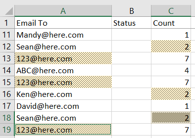
A use case that involves sending emails to a 3rd party person. I can determine how many emails I have sent out to a particular person by using the COUNTIF (or COUNTIFS) function in Excel.
But at the same time, I would like to know if it's possible to simply highlight the cells that have the same values as the current active cell.
Given an example below:
If I have the active cell at A19, can the cell A13, A15 and A19, and the rest of them with the same value be highlighted with a different color format?
I'm not too sure if there's a better way, but at this juncture, I came to a solution by using the Macro codes below:
Private Const MAX_CELL_SELECT_CNT As Integer = 100
'This code must go in the code pane of the worksheet being watched
Private Sub Worksheet_SelectionChange(ByVal Target As Range)
Dim rng As Range, r As Range, t As Range
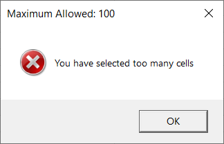
If Target.Cells.CountLarge > MAX_CELL_SELECT_CNT Then
MsgBox "You have selected too many cells", vbCritical, "Maximum Allowed: " & MAX_CELL_SELECT_CNT
Exit Sub
End If
Application.EnableEvents = False
Application.StatusBar = "Please wait while processing ..."
DoEvents
With ActiveSheet.Cells.Interior
.Pattern = xlNone
.PatternColorIndex = xlNone
.ThemeColor = xlNone
.TintAndShade = 0
.PatternTintAndShade = 0
End With
Set rng = Intersect(ActiveSheet.UsedRange, Target.EntireColumn)
If Not rng Is Nothing Then
For Each r In rng
For Each t In Target
If Trim(r.Value) <> "" And Trim(t.Value) <> "" And r.Value = t.Value Then
With r.Interior
.Pattern = xlGray16
.PatternColorIndex = xlAutomatic
.ThemeColor = xlThemeColorAccent4
.TintAndShade = 0.799981688894314
.PatternTintAndShade = 0
End With
End If
Next
DoEvents
Next
End If
Target.Activate
Application.StatusBar = ""
Application.EnableEvents = True
End SubThis approach seems to be working well and created the effect I wanted.
Selecting multiple cells is also supported with the same codes above.
NOTE:
i) I have built the logic so that empty cells will not be selected.
ii) I have set a Constant MAX_CELL_SELECT_CNT in the codes to set a threshold so that we can control the number of values to be looked up and prevent a heavy load such as in a scenario when one whole or multiple columns were being selected.
iii) DoEvents function was being added in the code so that we have a chance to pause the long process, just in case we did not handle it properly.
Hopefully, this article is useful to you.
You are encouraged and welcome to give me feedback for any possible improvements.

The best way to learn is to teach
Have a question about something in this article? You can receive help directly from the article author. Sign up for a free trial to get started.
Comments (1)
Commented: